3.2. The cosmological models
A few models are already implemented. I give a brief description below,
with references for works that discuss some of them in detail and works that
analyzed them with this code.
The models are objects created from the cosmic_objects.CosmologicalSetup class.
This class has a generic module solve_background that calls the Fluid’s
module rho_over_rho0 of each fluid to obtain the solution for their energy
densities.
When a solution cannot be obtained directly (like in some interacting models),
a fourth-order Runge-Kutta integration is done using the function
generic_runge_kutta from EPIC.utils’s integrators and the fluids`
drho_da.
There is an intermediate function get_Hubble_Friedmann to calculate the
Hubble rate either by just summing the energy densities, when called from the
Runge-Kutta integration, or calculating them with rho_over_rho0.
Some new models can be introduced in the code just by editing the
model_recipes.ini, available_species.ini and (optionally)
default_parameter_values.ini configuration files, without needing to
rebuild and install the EPIC’s package.
The format of the configuration .ini files is pretty straightforward and
the containing information can serve as a guide for what needs to be defined.
The \(\Lambda\text{CDM}\) model
When baryons and radiation are included, the solution to this cosmology will
require values for the parameters
\(\Omega_{c0}\),
\(\Omega_{b0}\),
\(T_{\text{CMB}}\),
\(H_0\),
or
\(h\),
\(\Omega_{c0} h^2\),
\(\Omega_{b0} h^2\),
\(T_{\text{CMB}}\),
and will find \(\Omega_{\Lambda} = 1 - \left( \Omega_{c0} + \Omega_{b0} + \Omega_{r0} \right)\) or
\(\Omega_{\Lambda} h^2 = h^2 - \left( \Omega_{c0} h^2 + \Omega_{b0} h^2 + \Omega_{r0} h^2 \right)\)
if physical. [1]
The radiation density parameter \(\Omega_{r0}\) is calculated according to
the CMB temperature \(T_{\text{CMB}}\), including the contribution of the
neutrinos (and antineutrinos) of the standard model.
Extending this model to allow curvature is not completely supported yet. The
Friedmann equation is
or
\(H_0\) is in units of \(\text{km s$^{-1}$ Mpc$^{-1}$}\).
This model is identified in the code by the label lcdm.
The \(w\text{CDM}\) model
Identified by wcdm, this is like the standard model except that the dark
energy equation of state can be any constant \(w_d\), thus having the
\(\Lambda\text{CDM}\) model as a specific case with \(w_d = -1\).
The Friedmann equation is like the above but with the dark energy contribution
multiplied by \((1+z)^{3(1+w_d)}\).
The Chevallier-Polarski-Linder parametrization
The CPL parametrization [2] of the dark energy equation of state
is also available. In this case, the dark energy contribution in the Friedmann equation is multiplied by \(\left(1 + z \right)^{3\left(1 + w_0 + w_a\right)} e^{-3 w_a z /\left(1 + z\right)}\) or \(a^{-3\left(1 + w_0 + w_a\right)} e^{-3 w_a \left(1 - a\right)}\), in terms of the scale factor.
The Barboza-Alcaniz parametrization
The Barboza-Alcaniz dark energy equation of state parametrization [3]
is implemented. This models gives a dark energy contribution in the Friedmann equation that is multiplied by the term \(x^{3(1+w_0)} \left( x^2 - 2 x + 2 \right)^{-3 w_1/2}\), where \(x \equiv 1/a\).
The Jassal-Bagla-Padmanabhan parametrization
Starting with version 1.4, the JBP parametrization [4] of the equation of state
can also be used. In this case, \(a^{-3\left(1 + w_0\right)} e^{- 3 w_1 \left[a\left(1 - a/2\right) - 1/2\right]}\) or \((1+z)^{3\left(1+w_0\right)} e^{3 w_1 z^2/2 \left(1+z\right)^2}\) is the term that goes into the dark energy contribution in the Friedmann equation.
Interacting Dark Energy models
A comprehensive review of models that consider a possible interaction between dark energy and dark matter is given by Wang et al. (2016) [5]. In interacting models, the individual conservation equations of the two dark fluids are violated, although still preserving the total energy conservation:
The shape of \(Q\) is what characterizes each model. Common forms are proportional to \(\rho_c\), to \(\rho_d\) (both supported) or to some combination of both (not supported in this version).
To create an instance of a coupled model (cde) with
\(Q \propto \rho_c\), use:
The mandatory species are idm and ide. You can add baryons
in the optional_species list keyword argument, but note that
matter is not available as a combined species for this model type
since dark matter is interacting with another fluid while baryons are
not. What is new here is the interaction_setup dictionary. This is
where we tell the code which species are interacting (at the moment
only an energy exchange within a pair is supported), to which of them
(idm) we associate the interaction parameter xi, indicate
the second one (ide) as having an interaction term proportional to
the other (idm) and specify the sign of the interaction term for
each fluid, in this case that means \(Q_c = 3 H \xi \rho_c\) and
\(Q_d = - 3 H \xi \rho_c\).
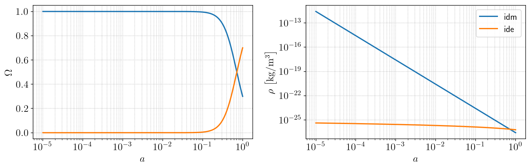
Here, I am exaggerating the value of the interaction parameter so we can
see a variation on the dark energy density that is due to the
interaction, not the equation-of-state parameter, which is \(-1\).
This same cosmology can be realized with the model type cde_lambda
without specifying the parameter wd, since the ilambda fluid has
fixed \(w_d = -1\). The dark matter interacting term \(Q_c\) is
positive with \(\xi\) positive, thus the lowering of the dark energy
density as its energy flows towards dark matter.
Fast-varying dark energy equation-of-state models
Models of dark energy with fast-varying equation-of-state parameter have been studied in some works [6]. Three such models were implemented as described in Marcondes and Pan (2017) [7]. We used this code in that work. They have all the density parameters present in the \(\Lambda\text{CDM}\) model besides the dark energy parameters that we describe in the following.
The Linder-Huterer parametrization (Model 1)
The model lh has the free parameters
\(w_p\),
\(w_f\),
\(a_t\) and
\(\tau\) characterizing the equation of state [8]
\(w_p\) and \(w_f\) are the asymptotic values of \(w_d\) in the past (\(a \to 0\)) and in the future (\(a \to \infty\)), respectively; \(a_t\) is the scale factor at the transition epoch and \(\tau\) is the transition width. The Friedmann equation is
where
The Felice-Nesseris-Tsujikawa parametrization (Model 2)
This FNT model fv2 alters the previous model to allow the dark energy
to feature an extremum value of the equation of state: [6]
where \(w_0\) is the current value of the equation of state and the other parameters have the interpretation as in the previous model. The Friedmann equation is
with
The Felice-Nesseris-Tsujikawa parametrization (Model 3)
Finally, we have another FNT model fv3 with the same parameters as in Model 2 but with equation of state [6]
It has a Friedmann equation identical to Model 2’s except that \(f_2(a)\) is replaced by
Footnotes
| [1] | That is, assuming derived=lambda, but we could also have done, for example, physical=False, derived=matter, specify \(\Omega_{\Lambda}\) and the code would get \(\Omega_{m0} = 1 - \left( \Omega_{\Lambda} + \Omega_{r0} \right)\) or, still, without specifying the derived parameter and with physical true, specify all the fluids’ density parameters and get \(h = \sqrt{\Omega_{c0} h^2 + \Omega_{b0} h^2 + \Omega_{r0} h^2 + \Omega_{\Lambda} h^2}\). |
| [2] | Chevallier M. & Polarski D., “Accelerating Universes with scaling dark matter”. International Journal of Modern Physics D 10 (2001) 213-223; Linder E. V., “Exploring the Expansion History of the Universe”. Physical Review Letters 90 (2003) 091301. |
| [3] | Barboza E. M. & Alcaniz J. S., “A parametric model for dark energy”. Physics Letters B 666 (2008) 415-419. |
| [4] | Jassal H. K., Bagla J. S., Padmanabhan T., “WMAP constraints on low redshift evolution of dark energy”. Monthly Notices of the Royal Astronomical Society 356 (2005) L11-L16; Jassal H. K., Bagla J. S., Padmanabhan T., “Observational constraints on low redshift evolution of dark energy: How consistent are different observations?”. Physical Review D 72 (2005) 103503. |
| [5] | Wang B., Abdalla E., Atrio-Barandela F., Pavón D., “Dark matter and dark energy interactions: theoretial challenges, cosmological implications and observational signatures”. Reports on Progress in Physics 79 (2016) 096901. |
| [6] | (1, 2, 3) Corasaniti P. S. & Copeland E. J., “Constraining the quintessence equation of state with SnIa data and CMB peaks”. Physical Review D 65 (2002) 043004; Basset B. A., Kunz M., Silk J., “A late-time transition in the cosmic dark energy?”. Monthly Notices of the Royal Astronomical Society 336 (2002) 1217-1222; De Felice A., Nesseris S., Tsujikawa S., “Observational constraints on dark energy with a fast varying equation of state”. Journal of Cosmology and Astroparticle Physics 1205, 029 (2012). |
| [7] | Marcondes R. J. F. & Pan S., “Cosmic chronometer constraints on some fast-varying dark energy equations of state”. arXiv:1711.06157 [astro-ph.CO]. |
| [8] | Linder E. V. & Huterer D., “How many dark energy parameters?”. Physical Review D 72 (2005) 043509. |