4.4. MCMC from the GUI

Starting with version 1.3, the simulations can also be performed from the graphical interface. Run:

$ epic.py

to launch EPIC’s graphical interface. When you choose and set up a model, instead of specifying the values of the model parameters, you can now also infer them using MCMC directly from this interface, where you can define the priors and choose the datasets to be used.

Select the tab “Constrain with MCMC” in the bottom frame. Note that this area is made of three sections. The left panel is where the priors are defined. It is populated with the free parameters of the selected model after the model is built. The first column sets the priors, which can be flat or Gaussian, with two parameters defining these distributions. The entries are automatically filled with default values that the user should change as needed. Another option is to fix the parameter and indicate the fixed value. By default all priors are set to flat, except the prior of the CMB temperature when radiation is included, which is fixed but can also be changed. The second column defines the square root of the variance of each parameter, to compose a diagonal covariance matrix for the proposal function. The third column shows the units of the quantities, when it is the case.

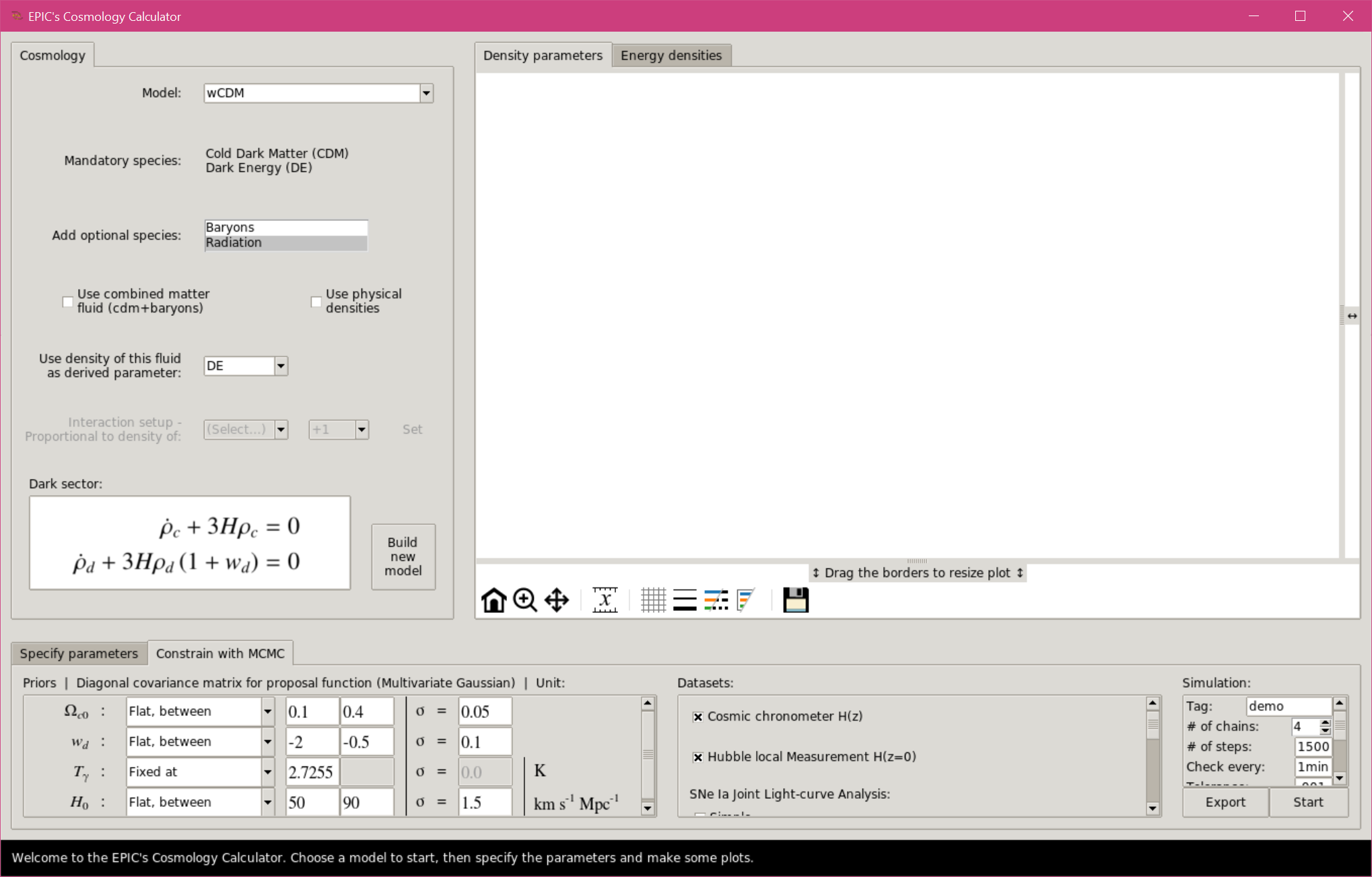
MCMC with the Graphical User Interface.

The middle panel is where the user can choose which datasets to include in the comparison (see section The datasets). Note that BAO and CMB data are only available when the model includes baryons and radiation. The JLA dataset (simple or full) will add more parameters to the analysis. The priors for these nuisance parameters must as well be defined by the user.

Finally, the right panel defines options for the simulation, such as a tag for the folder where the output will be saved, the number of chains, the number of steps to be run in each loop, the time interval to check for convergence (and display the plots), the tolerance for the convergence check, the desired interval for the acceptance rates (which determines when chains should be discarded), the number of sigma confidence levels to display in the plots and report in the final output table, the number of bins for the histograms shown during the evolution. Next, there are toggles to set whether or not, after finishing the simulation, a last analysis with the --kde option should be made, save the plots in .png besides .pdf (always saved) and to use a proposal covariance matrix (which need not be diagonal) imported from a text file. There are also buttons enabling plot customization options much like those available to the Cosmology Calculator. All changes of style are applied to existing plots, which also affect any other plots of the Cosmology Calculator (energy densities, density parameters or distances) that the user may already have generated previously if the selected option is available in the corresponding Calculator menus in the “Specify Parameters” tab.

The “Export” button prepares a .ini file based on these settings and can also be used to run MCMC from the terminal (instructions are given in the header of the .ini file). The “Start” button exports the .ini file and starts the simulation right away, after the user have informed the location to save the file. When the simulation starts, a terminal output is shown in a new tab “Output” in the bottom frame. Also shown are the acceptance rates, the number of accepted states of each chain (as the data are saved to the disk at each loop) and the normal fits to the marginalized distributions (when convergence is checked).

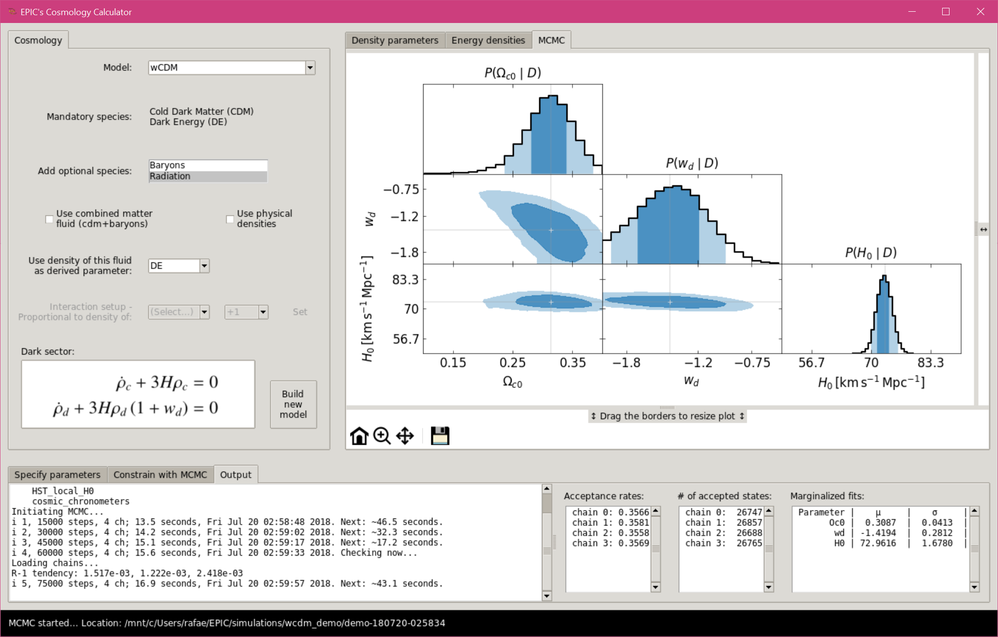
MCMC with the Graphical User Interface, simulation running.

When finished, the plot is done again using ranges automatically adapted for optimal view and can be further customized.

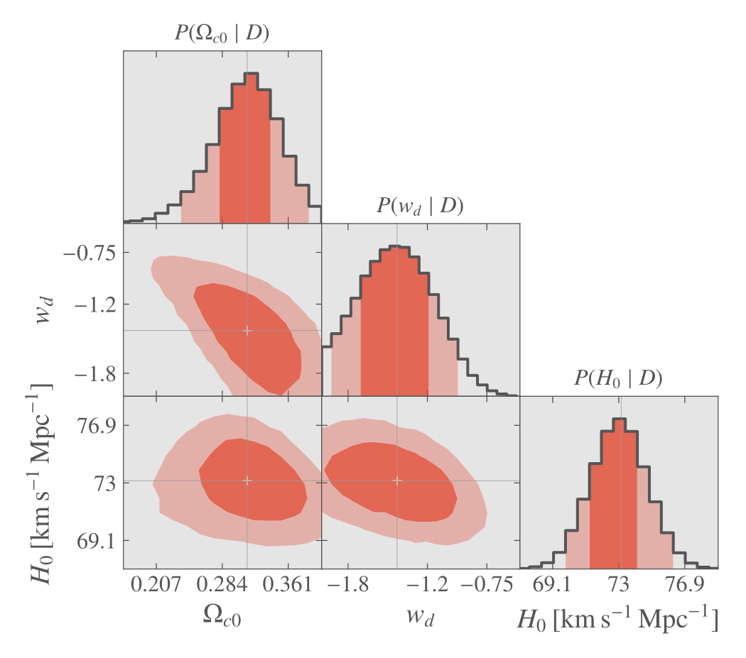
MCMC with the Graphical User Interface, final plot.