4.5. Running PT-MCMC
Alternatively, we can use the Parallel Tempering algorithm. This is specially useful when the posterior distribution is likely to present more than one peak and these peaks are well separated. In such cases, the standard MCMC sampler is not efficient and may even fail to detect peaks away from where the chain begun. With Parallel Tempering, the ground-temperature chain that samples the true posterior distribution is more likely to jump between separate peaks, more efficiently visiting the entire parameter space. This is possible thanks to a mechanism providing state exchange between chains following a temperature ladder, in which the posterior is progressively flattened so as to reduce the differences of probability density amplitude that otherwise would keep the chains locally stuck.
In order to illustrate the potential of this method, we will run a PT-MCMC on
an artificial distribution. A test model is created with a likelihood given as
a combination of various univariate Gaussian distributions. We will see in the
following how we are able to recover the exact marginalized posterior
distributions.
The function reserved for this is the disttest in the likelihood.py file.
In our example, this model has three free parameters, \(a, b, c\), all with
flat priors between 0 and 1. The likelihood consists of the Gaussian functions
\(N_a(0.5, 0.01)\), \(N_b(0.2, 0.03)\) and two Gaussian functions for
the third parameter, \(N_c(0.3, 0.02)\) and \(N_c(0.75, 0.02)\),
giving two distant peaks several sigmas apart, with respective weights
\(0.7, 0.3\).
Initializing the chains
This works pretty much in the same way as the previous method. Just run:
python initialize_chains.py disttest.ini chains=4 mode=PT
mode=PT is mandatory to specify that you want to use PT and not the
default sampler, standard MCMC.
You will be prompted about after how many steps the algorithm should propose a
state swap:
Please specify after how many steps should propose a swap: 30
or you can bypass the information with nswap=30.
At every step a random number \(u\) between 0 and 1 is generated and a
swap will be proposed if \(u < 1/n_s\).
The default temperature ladder is between \(\beta=1\) (ground chain) and
\(2^{10}\), evenly distributed over the log scale over the number of chains
given.
This can be changed with betascale=linear, for example (it will actually be
linear for whatever given value different than log) and betamax=6
(instead of 10), for example.
Sampling the posterior distribution
Next, we run as we would a standard MCMC set of chains:
python epic.py <FULL-PATH-TO>/disttest/PT-171022-185848/ steps=3000 limit=90000
Unlike the standard method, convergence will not be checked automatically
(remember only the ground temperature chain corresponds to the true posterior
distribution).
We thus need to specify a limit so it stops after some large number of
states.
Because the higher-temperature distributions are wider, in this code
I try to guarantee an efficient sampling for all chains by dividing
the variances in the proposal function in each chain by their
respective value of \(\beta\).
Analyzing the chains
In the PT method, convergence is not assessed automatically, since each
chain has a different temperature, thus not sampling from the same
distribution.
We could think of comparing the different chains after taking the frequencies
of each bin to the power \(1/\beta\), but I believe this could lead to
inaccuracies due to statistical noise amplification in the higher-temperature
chains, so I have not tested nor implemented this yet.
In order to determine if you can already stop evolving your chains, I recommend
running a second similar simulation so you can compare the ground temperature
chains of the two (or more, but two is enough). To do this, create and run a
second simulation with:
python epic.py disttest.ini chains=4 mode=PT steps=9000 limit=90000 nswap=30
and then:
python analyze.py <FULL-OR-RELATIVE-PATH-TO-FIRST-SIMULATION> calculate_R=<FULL-OR-RELATIVE-PATH-TO-SECOND-SIMULATION>
You can do this at any time while the simulations are still running, even if
they have different lengths. The only requirement is that the one in the
calculate_R argument is the longer one.
The minimum of the lengths of the two ground temperature chains will be used,
the rest is disregarded.
The directory of the main argument (the shorter chain) will contain the convergence results.
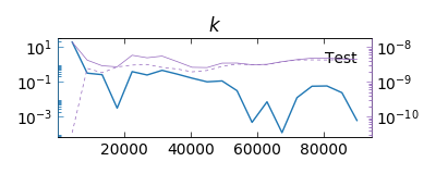
Convergence between two chains from two Parallel Tempering simulations.
During the simulation, the code will print the acceptance rates of the chains
every 10 iterations.
The acceptance rate of the ground temperature chain and the swap rate are
printed every iteration.
After limit steps, the code outputs the Akaike and Bayesian information
criteria, AIC and BIC, and generates the usual plots.
Analyzing the resulting posterior and even checking convergence is fast since
only the ground temperature chains need to be loaded.
However, since this is Parallel Temperature, we can use the information of the
higher-temperature chains to compute the Bayesian evidence, we just need to
specify that we want so with the option evidence. If we ask to
plot_sequences or the correlations (with ACF), since all chains will
have to be loaded the evidence will also be computed anyway even without the
argument evidence.
It is interesting to inspect the sequences of the different temperatures. We
can clearly see the jumps between the peaks occurring in the lower-temperature
chains and the good mixing of the high-temperature chains, where the peaks are
smoothed out.
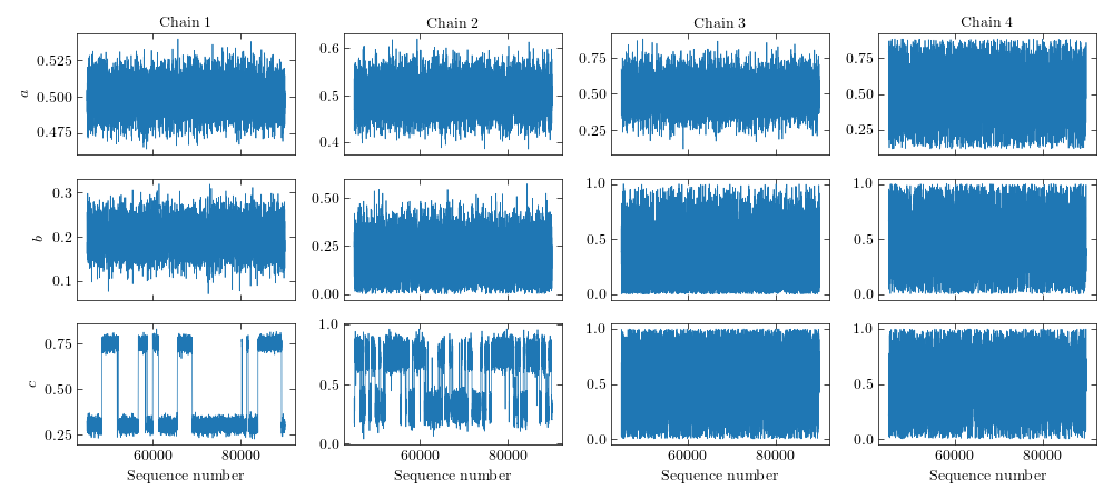
Sequences of a Parallel Tempering MCMC simulation
The evidence is calculated from the area under the following curve
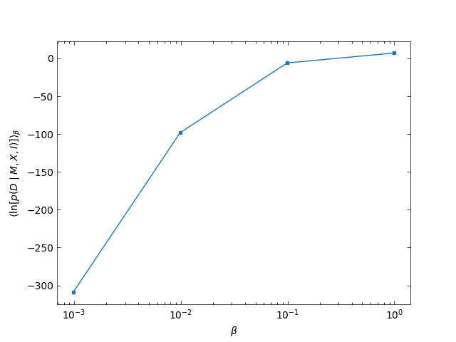
Log-evidence calculated by thermo-integration of the PT chains.
Of course, the more chains we use the more precise this calculation will be. So let us now see how accurate is our simulation. In the following triangle plot, we show the exact curves of the Gaussian distributions superposing the histograms.
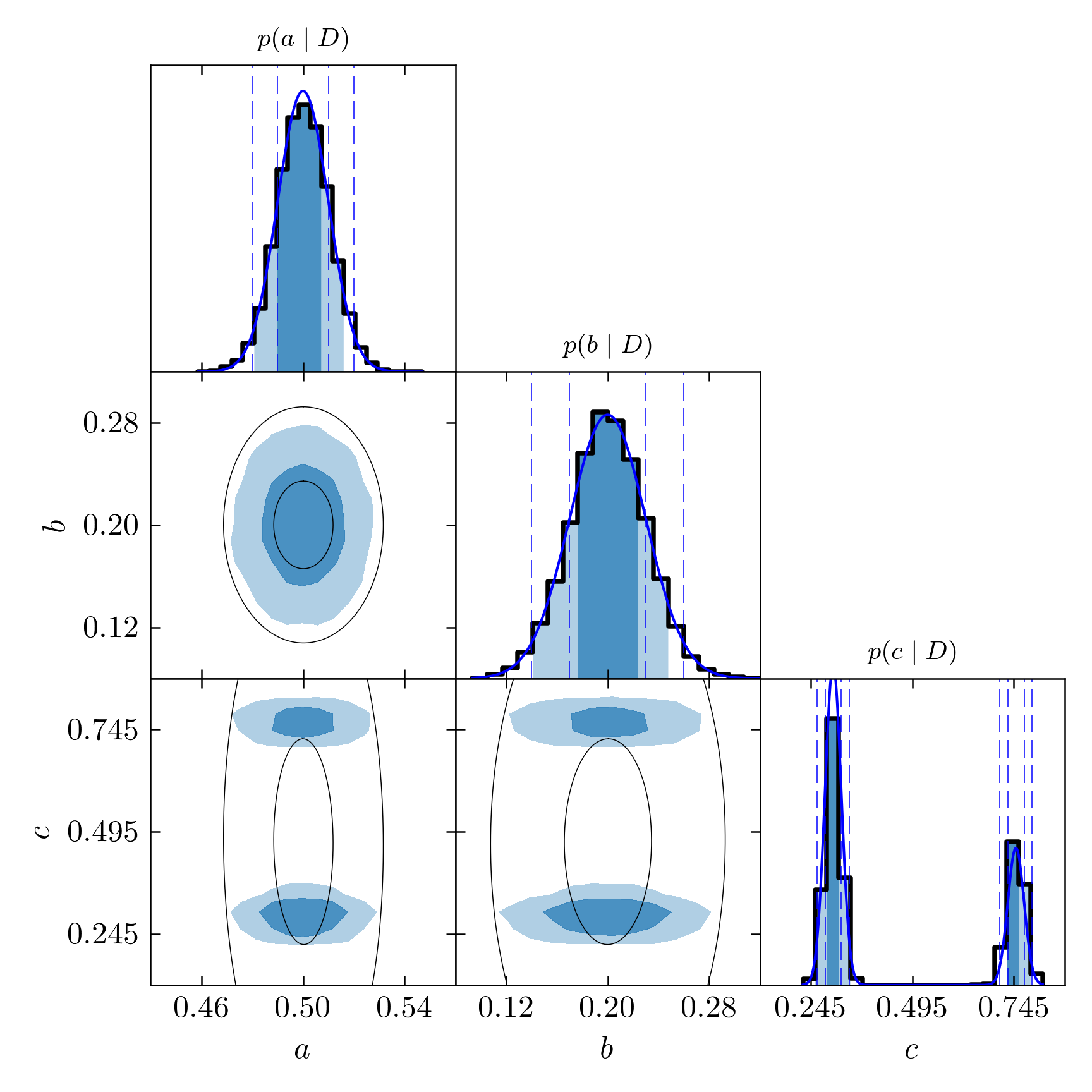
Triangle plot for the PT simulation with the true marginalized probabilities in blue.
Notice how the resulting histograms approximate very well the true functions, including the separated peaks given by the sum of two Gaussians. In standard MCMC, we would very probably obtain only one of the peaks. Which one depends on where the chain starts.
Let us improve this a little. These histograms with 20 bins are ok for the
first two the parameters, but because of the wider range of data along the
\(c\) axis, it is too little.
Using a higher number of bins helps but most bins would be wasted since the
division spans uniformly over the entire range of data and there are practically
no points inside a large interval between the two peaks.
The standard kernel density estimates with the bandwidth tuned for
Gaussian-like distributions does not work well with multi-peaked distributions
because the standard deviation will be rather large. We circumvented this
limitation in this program by allowing the calculation of KDE on separate
subsets of data. For this case, instead of running make_kde([array,]) we
can do make_kde([array[array < 0.5], array[array > 0.5]]), since the peak
separation is very clear and there will probably be no points above
\(c=0.5\) belonging to the first peak and no points below this value
belonging to the second peak (when the peaks are closer together this may be
much more complicated to accomplish). This will make KDE for the two subsets
separately and then join them together again, resulting in an accurate
representation of the data.
The make_kde function already receives a list of arrays to make this
possible when we have separate arrays of data. In this case, we just need to
tell the program where to split the single array in two. This is done by saving a file disttest.true_fit containing the weight, \(\mu\) and \(\sigma\) parameters of the separated true distributions (only Gaussian is supported):
1       0.5     0.01
1       0.2     0.03
0.7     0.3     0.02    0.3     0.75    0.02
Notice how the KDE curves match very well the true functions, in blue lines:
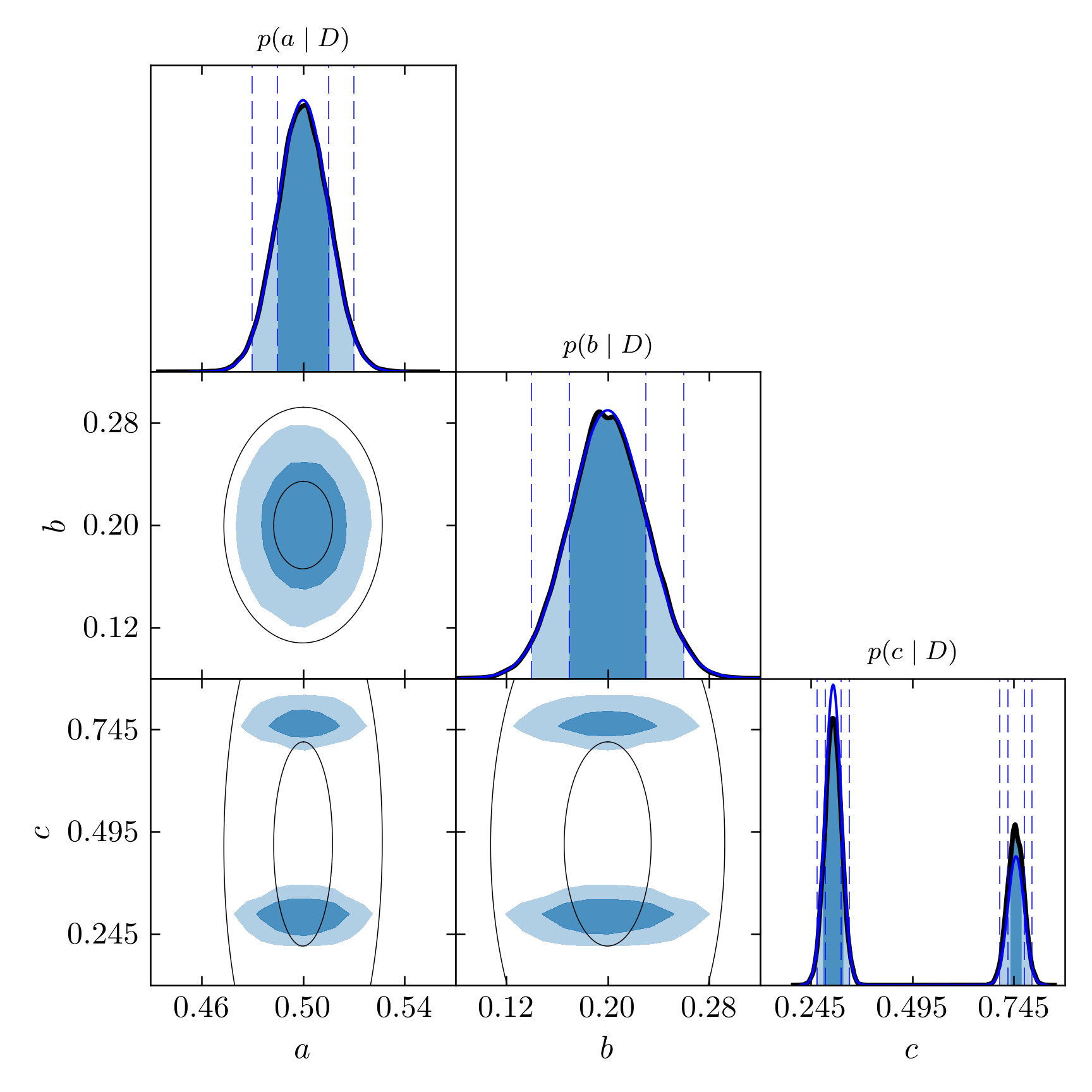
Triangle plot for the PT simulation with KDE smoothed distributions and true density probabilities.
The confidence levels are extracted from this marginalized distributions. The precision in the determination of the intervals is then limited by the resolution of the histograms (the number of bins). I recommend using KDE whenever is possible. Using more bins is also an option but requires having very long chains so this number can be raised considerably. KDE provides very good precision without needing too much data points (as long as there is enough for the chains to have converged). It is clear from these images how the KDE curves match much better \(1\sigma\) and \(2\sigma\) confidence intervals. The shaded regions are not expected to match the dashed lines in the marginalized distribution of the third parameter (unless the two Gaussians had equal weights and widths), however, as they are calculated globally rather than locally.
At this moment, more than two separated peaks are not supported for this
splitting by the analyze.py routine, although it can be done directly with
any number of separated arrays in a list in the make_kde function.
Finally, let us see the results from this simulation. The image below is a screenshot of the kde_table.pdf file obtained compiling the kde_table.tex file saved in the kde_estimates directory:
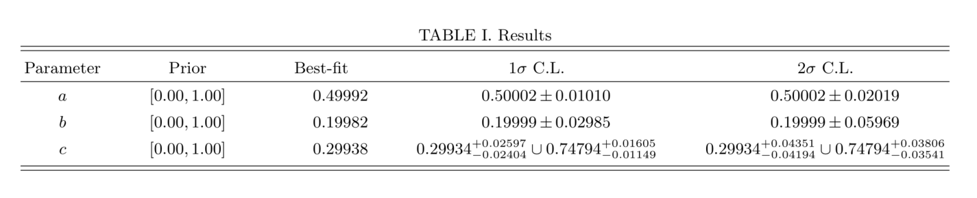
Summary of the results of our analysis with the test distribution.
Since the parameter \(c\) has two peaks of high density probability, the
resulting confidence regions are composed of two intervals. The union symbol
\(\cup\) is used to represent this configuration. The result for the
parameter \(b\) may look different from the true Gaussian function because
of an artifact in the peak, showing doubled tips. The reported result considers
the highest of the tips as the central value, the error bars being calculated
from that value. For cases like this, it is interesting to simply report the
Gaussian fits instead. They can be inserted automatically in the tables if we
save a file named normal_kde.txt in the simulation directory informing the
name of the parameters (one per line) that look Gaussian. Then the mean and
standard deviation will be printed in the table when drawhistograms.py is
run again. This has been done for the result shown above.
Adaptation (beta)
An adaptive routine is implemented following the ideas in Łącki & Miasojedow 2016 [1], but this needs more tests and is still in beta. Come back later to check.
| [1] | Łącki M. K. & Miasojedow B. “State-dependent swap strategies and automatic reduction of number of temperatures in adaptive parallel tempering algorithm”. Statistics and Computing 26, 951–964 (2016). |